Apply GraphVelo to HCMV dataset

In this tutorial, we will show how to incorporate GraphVelo with current dynamo workflow.

GraphVelo is able to infer the kinetic factors which do not undergoing splicing events using RNA velocity.

[1]:

import numpy as np
import pandas as pd
import scanpy as sc
import dynamo as dyn

import seaborn as sns
import matplotlib.pyplot as plt
%matplotlib inline

import warnings
warnings.filterwarnings("ignore")

[2]:

import graphvelo
from graphvelo.plot import gene_trend
from graphvelo.graph_velocity import GraphVelo

Load data file

You can also get access to it via https://drive.google.com/file/d/1E_gpsRRuTrrIX8qX4biPejzjiKbD5hKd/view?usp=drive_link

You can download the adata file via https://drive.google.com/file/d/1uH5HJ7EqjnF94oovxxCYuB4-Oc6gKBgt/view?usp=drive_link

[3]:

gtf_data = graphvelo.datasets.hcmv_annot()
gtf_data[8] = gtf_data[8].str.extract(r'gene_id "([^"]+)"')
viral_genes_names = gtf_data[8].unique()
viral_genes_names = np.delete(viral_genes_names, np.where(viral_genes_names=='UL38')) # Exclude 0 expression viral gene
len(viral_genes_names)

[3]:

[4]:

adata = sc.read('datasets/hcmv/hcmv_preprocessed.h5ad')
adata

[4]:

AnnData object with n_obs × n_vars = 1454 × 28051
    obs: 'orig.ident', 'nCount_RNA', 'nFeature_RNA', 'nCount_Protein', 'nFeature_Protein', 'batch', 'percent.mt', 'Demultiplex', 'TotalVir', 'TotalVirPercentage', 'CD45', 'HLA.DR', 'HCMV.Status', 'nCount_SCT', 'nFeature_SCT', 'SCT_snn_res.0.8', 'seurat_clusters', 'clusters', 'donor', 'Cluster.Type', 'annot'
    uns: 'genes_to_use'
    obsm: 'X_umap'
    layers: 'spliced', 'unspliced'

[5]:

host_genes = ~pd.Series(adata.var_names).isin(viral_genes_names.tolist()).values
viral_genes = pd.Series(adata.var_names).isin(viral_genes_names.tolist()).values
host_genes_names = adata.var_names[host_genes]
viral_genes_names = adata.var_names[viral_genes]

[6]:

valid_genes = list(viral_genes_names)+['IFNB1']  # Include IFNB1 which serves as an important host gene in the immune process

Standard dynamo preprocessing criteria

[7]:

dyn.pp.recipe_monocle(adata,
                      genes_use_for_norm=host_genes_names,
                      genes_to_append=valid_genes,
                      )

|-----? dynamo.preprocessing.deprecated is deprecated.
|-----> recipe_monocle_keep_filtered_cells_key is None. Using default value from DynamoAdataConfig: recipe_monocle_keep_filtered_cells_key=True
|-----> recipe_monocle_keep_filtered_genes_key is None. Using default value from DynamoAdataConfig: recipe_monocle_keep_filtered_genes_key=True
|-----> recipe_monocle_keep_raw_layers_key is None. Using default value from DynamoAdataConfig: recipe_monocle_keep_raw_layers_key=True
|-----> apply Monocole recipe to adata...
|-----> ensure all cell and variable names unique.
|-----> ensure all data in different layers in csr sparse matrix format.
|-----> ensure all labeling data properly collapased
|-----> filtering cells...
|-----> 1454 cells passed basic filters.
|-----> filtering gene...
|-----> 7661 genes passed basic filters.
|-----> calculating size factor...
|-----> selecting genes in layer: X, sort method: SVR...
|-----> size factor normalizing the data, followed by log1p transformation.
|-----> Set <adata.X> to normalized data
|-----> applying PCA ...
|-----> <insert> X_pca to obsm in AnnData Object.
|-----> cell cycle scoring...
|-----> computing cell phase...
|-----> [Cell Phase Estimation] completed [9.6253s]
|-----> [Cell Cycle Scores Estimation] completed [0.1075s]
|-----> [recipe_monocle preprocess] completed [3.3010s]

[8]:

dyn.tl.dynamics(adata)

|-----> dynamics_del_2nd_moments_key is None. Using default value from DynamoAdataConfig: dynamics_del_2nd_moments_key=False
|-----------> removing existing M layers:[]...
|-----------> making adata smooth...
|-----> calculating first/second moments...
|-----> [moments calculation] completed [6.5298s]

estimating gamma: 100%|██████████| 1999/1999 [00:14<00:00, 141.37it/s]

[8]:

AnnData object with n_obs × n_vars = 1454 × 28051
    obs: 'orig.ident', 'nCount_RNA', 'nFeature_RNA', 'nCount_Protein', 'nFeature_Protein', 'batch', 'percent.mt', 'Demultiplex', 'TotalVir', 'TotalVirPercentage', 'CD45', 'HLA.DR', 'HCMV.Status', 'nCount_SCT', 'nFeature_SCT', 'SCT_snn_res.0.8', 'seurat_clusters', 'clusters', 'donor', 'Cluster.Type', 'annot', 'nGenes', 'nCounts', 'pMito', 'pass_basic_filter', 'Size_Factor', 'spliced_Size_Factor', 'initial_cell_size', 'initial_unspliced_cell_size', 'initial_spliced_cell_size', 'unspliced_Size_Factor', 'ntr', 'cell_cycle_phase'
    var: 'nCells', 'nCounts', 'pass_basic_filter', 'score', 'log_m', 'log_cv', 'frac', 'use_for_pca', 'ntr', 'use_for_dynamics'
    uns: 'genes_to_use', 'pp', 'velocyto_SVR', 'PCs', 'explained_variance_ratio_', 'pca_mean', 'pca_fit', 'feature_selection', 'cell_phase_order', 'cell_phase_genes', 'vel_params_names', 'dynamics'
    obsm: 'X_umap', 'X_pca', 'X', 'cell_cycle_scores'
    varm: 'vel_params'
    layers: 'spliced', 'unspliced', 'X_unspliced', 'X_spliced', 'M_u', 'M_uu', 'M_s', 'M_us', 'M_ss', 'velocity_S'
    obsp: 'moments_con'

[9]:

dyn.tl.neighbors(adata)

|-----> Start computing neighbor graph...
|-----------> X_data is None, fetching or recomputing...
|-----> fetching X data from layer:None, basis:pca
|-----> method arg is None, choosing methods automatically...
|-----------> method ball_tree selected

[9]:

AnnData object with n_obs × n_vars = 1454 × 28051
    obs: 'orig.ident', 'nCount_RNA', 'nFeature_RNA', 'nCount_Protein', 'nFeature_Protein', 'batch', 'percent.mt', 'Demultiplex', 'TotalVir', 'TotalVirPercentage', 'CD45', 'HLA.DR', 'HCMV.Status', 'nCount_SCT', 'nFeature_SCT', 'SCT_snn_res.0.8', 'seurat_clusters', 'clusters', 'donor', 'Cluster.Type', 'annot', 'nGenes', 'nCounts', 'pMito', 'pass_basic_filter', 'Size_Factor', 'spliced_Size_Factor', 'initial_cell_size', 'initial_unspliced_cell_size', 'initial_spliced_cell_size', 'unspliced_Size_Factor', 'ntr', 'cell_cycle_phase'
    var: 'nCells', 'nCounts', 'pass_basic_filter', 'score', 'log_m', 'log_cv', 'frac', 'use_for_pca', 'ntr', 'use_for_dynamics'
    uns: 'genes_to_use', 'pp', 'velocyto_SVR', 'PCs', 'explained_variance_ratio_', 'pca_mean', 'pca_fit', 'feature_selection', 'cell_phase_order', 'cell_phase_genes', 'vel_params_names', 'dynamics', 'neighbors'
    obsm: 'X_umap', 'X_pca', 'X', 'cell_cycle_scores'
    varm: 'vel_params'
    layers: 'spliced', 'unspliced', 'X_unspliced', 'X_spliced', 'M_u', 'M_uu', 'M_s', 'M_us', 'M_ss', 'velocity_S'
    obsp: 'moments_con', 'distances', 'connectivities'

Apply GraphVelo to refine manifold-constrained velocity vectors

[10]:

gv = GraphVelo(adata, xkey='M_s', vkey='velocity_S')
gv.train()

Learning Phi in tangent space projection.: 100%|██████████| 1454/1454 [00:03<00:00, 373.41it/s]

[11]:

adata.layers['velocity_gv'] = gv.project_velocity(adata.layers['M_s'])
adata.obsm['gv_pca'] = gv.project_velocity(adata.obsm['X_pca'])
adata.obsm['gv_umap'] = gv.project_velocity(adata.obsm['X_umap'])

projecting velocity vector to low dimensional embedding: 100%|██████████| 1454/1454 [00:08<00:00, 168.14it/s]
projecting velocity vector to low dimensional embedding: 100%|██████████| 1454/1454 [00:00<00:00, 19916.19it/s]
projecting velocity vector to low dimensional embedding: 100%|██████████| 1454/1454 [00:00<00:00, 18743.85it/s]

[12]:

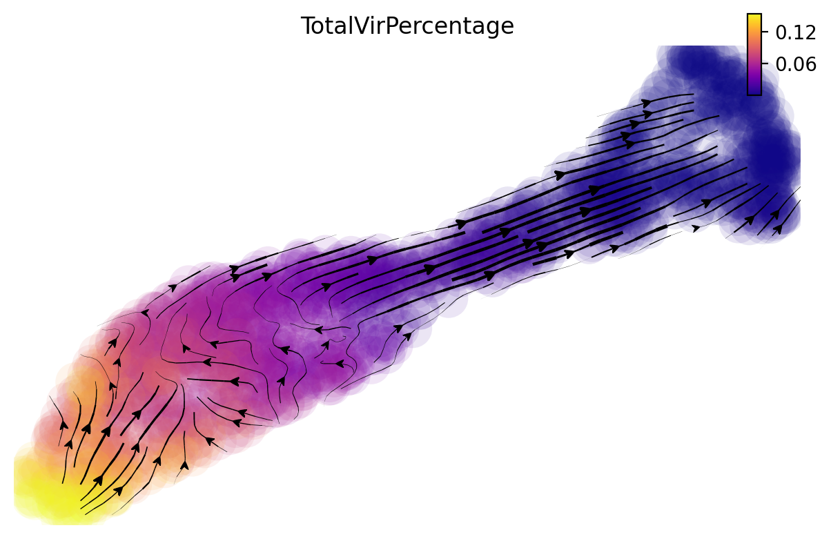
dyn.pl.streamline_plot(adata, color=['TotalVirPercentage'], vector='gv', cmap='plasma')

|-----> method arg is None, choosing methods automatically...
|-----------> method kd_tree selected
|-----------> plotting with basis key=X_umap

../../_images/graphvelo_notebooks_tutorials_tutorial_hcmv_16_1.png

[13]:

adata = adata[:, adata.var['use_for_pca']]
adata

[13]:

View of AnnData object with n_obs × n_vars = 1454 × 1999
    obs: 'orig.ident', 'nCount_RNA', 'nFeature_RNA', 'nCount_Protein', 'nFeature_Protein', 'batch', 'percent.mt', 'Demultiplex', 'TotalVir', 'TotalVirPercentage', 'CD45', 'HLA.DR', 'HCMV.Status', 'nCount_SCT', 'nFeature_SCT', 'SCT_snn_res.0.8', 'seurat_clusters', 'clusters', 'donor', 'Cluster.Type', 'annot', 'nGenes', 'nCounts', 'pMito', 'pass_basic_filter', 'Size_Factor', 'spliced_Size_Factor', 'initial_cell_size', 'initial_unspliced_cell_size', 'initial_spliced_cell_size', 'unspliced_Size_Factor', 'ntr', 'cell_cycle_phase'
    var: 'nCells', 'nCounts', 'pass_basic_filter', 'score', 'log_m', 'log_cv', 'frac', 'use_for_pca', 'ntr', 'use_for_dynamics'
    uns: 'genes_to_use', 'pp', 'velocyto_SVR', 'PCs', 'explained_variance_ratio_', 'pca_mean', 'pca_fit', 'feature_selection', 'cell_phase_order', 'cell_phase_genes', 'vel_params_names', 'dynamics', 'neighbors'
    obsm: 'X_umap', 'X_pca', 'X', 'cell_cycle_scores', 'gv_pca', 'gv_umap'
    varm: 'vel_params'
    layers: 'spliced', 'unspliced', 'X_unspliced', 'X_spliced', 'M_u', 'M_uu', 'M_s', 'M_us', 'M_ss', 'velocity_S', 'velocity_gv'
    obsp: 'moments_con', 'distances', 'connectivities'

[14]:

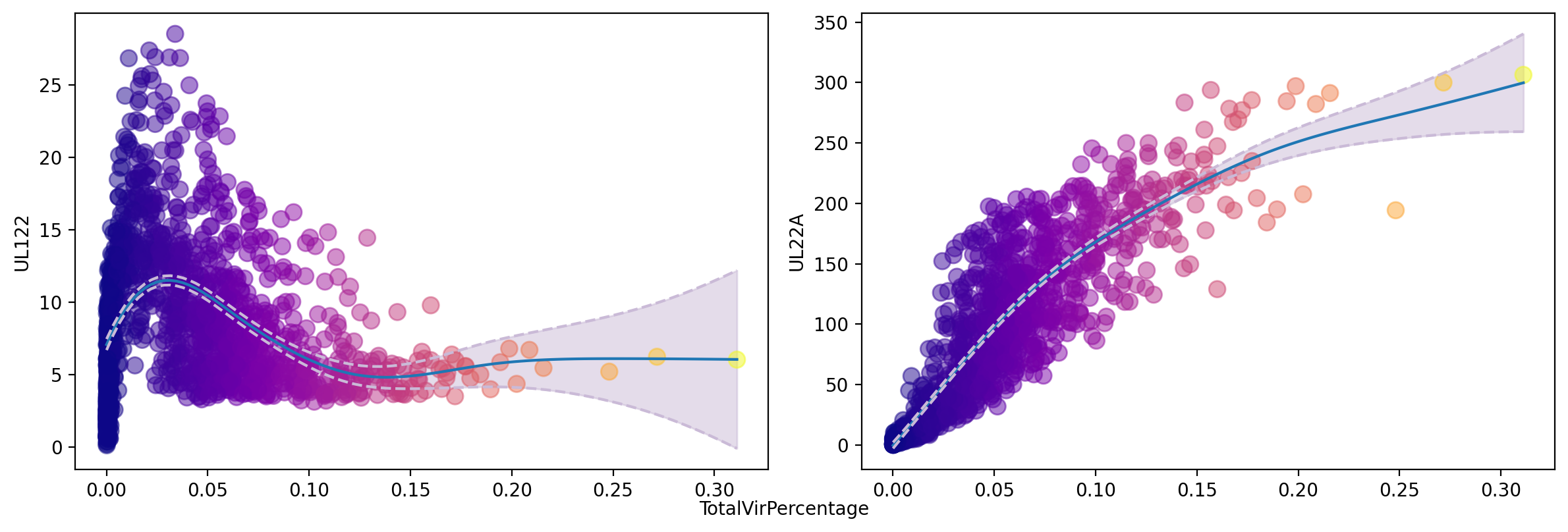
gene_trend(adata, ['UL122', 'UL22A'], layer='M_s', tkey='TotalVirPercentage', color='TotalVirPercentage', n_splines=8, pointsize=80)
plt.show()
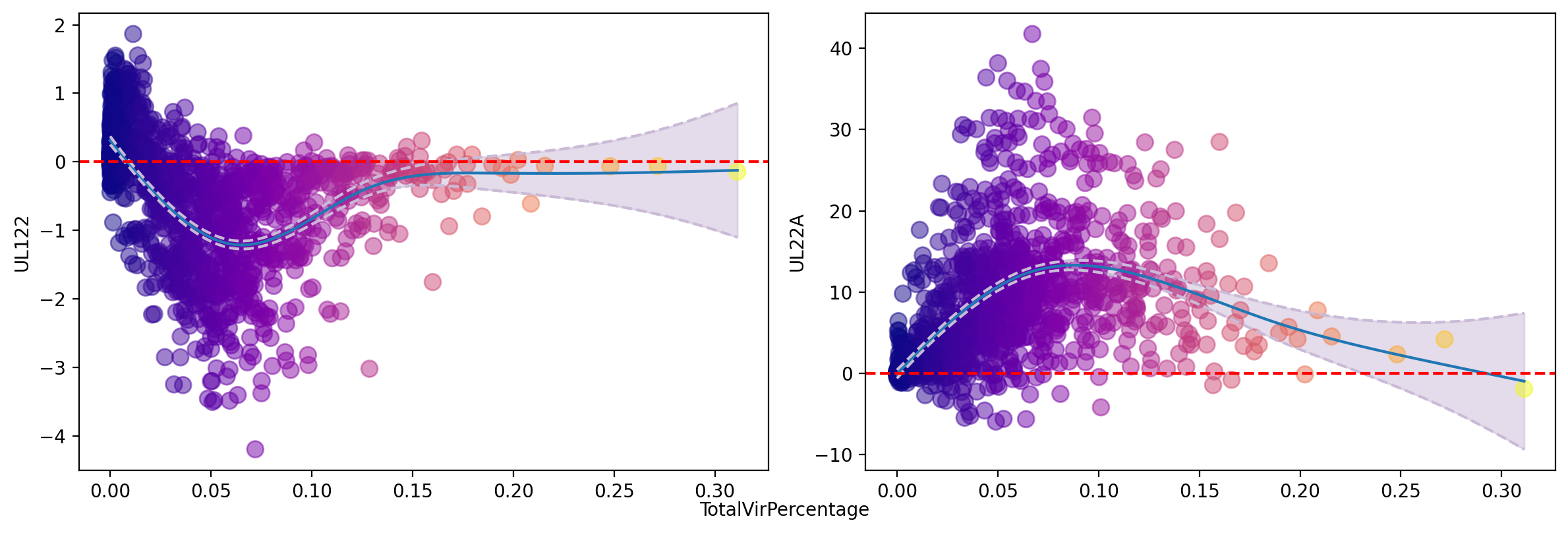
gene_trend(adata, ['UL122', 'UL22A'], layer='velocity_gv', tkey='TotalVirPercentage', color='TotalVirPercentage', zero_indicator=True, n_splines=8, pointsize=80)
plt.show()

Fitting trends using GAM:   0%|          | 0/2 [00:00<?, ?it/s]Fitting trends using GAM: 100%|██████████| 2/2 [00:00<00:00, 42.03it/s]

../../_images/graphvelo_notebooks_tutorials_tutorial_hcmv_18_1.png

Fitting trends using GAM: 100%|██████████| 2/2 [00:00<00:00, 22.52it/s]

../../_images/graphvelo_notebooks_tutorials_tutorial_hcmv_18_3.png

Working with dynamo vector field analyses

[15]:

adata.obsm['velocity_umap'] = adata.obsm['gv_umap'].copy()
dyn.vf.VectorField(adata, basis='umap', M=100, pot_curl_div=True)

|-----> VectorField reconstruction begins...
|-----> Retrieve X and V based on basis: UMAP.
        Vector field will be learned in the UMAP space.
|-----> Generating high dimensional grids and convert into a row matrix.
|-----> Learning vector field with method: sparsevfc.
|-----> [SparseVFC] begins...
|-----> Sampling control points based on data velocity magnitude...
|-----> method arg is None, choosing methods automatically...
|-----------> method kd_tree selected
|-----> [SparseVFC] completed [11.0037s]
|-----> Running ddhodge to estimate vector field based pseudotime in umap basis...
|-----> graphizing vectorfield...
|-----------? nbrs_idx argument is ignored and recomputed because nbrs_idx is not None and return_nbrs=True
|-----------> calculating neighbor indices...
|-----> method arg is None, choosing methods automatically...
|-----------> method kd_tree selected
|-----> [ddhodge completed] completed [10.3228s]
|-----> Computing curl...

Calculating 2-D curl: 100%|██████████| 1454/1454 [00:00<00:00, 27264.60it/s]

|-----> Computing divergence...


Calculating divergence: 100%|██████████| 2/2 [00:00<00:00, 90.93it/s]

|-----> [VectorField] completed [21.4902s]

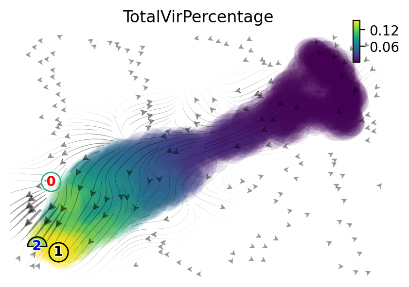
[16]:

fig, ax = plt.subplots(figsize=(5,4))
ax = dyn.pl.topography(adata, n=20,
                       color='TotalVirPercentage', ax=ax,
                       save_show_or_return='return',
                       color_key_cmap='plasma',)
ax.set_aspect(0.8)
plt.show()

|-----> Vector field for umap is but its topography is not mapped. Mapping topography now ...
|-----> method arg is None, choosing methods automatically...
|-----------> method kd_tree selected
|-----------> plotting with basis key=X_umap

../../_images/graphvelo_notebooks_tutorials_tutorial_hcmv_21_1.png

[17]:

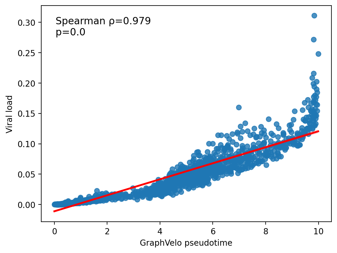
df = adata.obs[['umap_ddhodge_potential', 'TotalVirPercentage']]
df.columns = ['GraphVelo pseudotime', 'Viral load']

import scipy
res = scipy.stats.spearmanr(df['GraphVelo pseudotime'], df['Viral load'])
ax = sns.regplot(df, x='GraphVelo pseudotime', y='Viral load', line_kws=dict(color="r"))
ax.text(0.05, 0.95, s=f'Spearman \u03C1={res[0]:.3f}\np=0.0', transform=ax.transAxes, fontsize=12, color='black', verticalalignment='top')
# plt.savefig('figures_v2/graphvelo_time.pdf', format='pdf', dpi=300)
plt.show()

../../_images/graphvelo_notebooks_tutorials_tutorial_hcmv_22_0.png

Working with dynamo perturbation analyses

[18]:

adata.obsm['velocity_pca'] = adata.obsm['gv_pca'].copy()
dyn.vf.VectorField(adata, basis='pca', M=500)

|-----> VectorField reconstruction begins...
|-----> Retrieve X and V based on basis: PCA.
        Vector field will be learned in the PCA space.
|-----> Learning vector field with method: sparsevfc.
|-----> [SparseVFC] begins...
|-----> Sampling control points based on data velocity magnitude...
|-----> method arg is None, choosing methods automatically...
|-----------> method ball_tree selected
|-----> [SparseVFC] completed [4.3348s]
|-----> [VectorField] completed [4.4279s]

[19]:

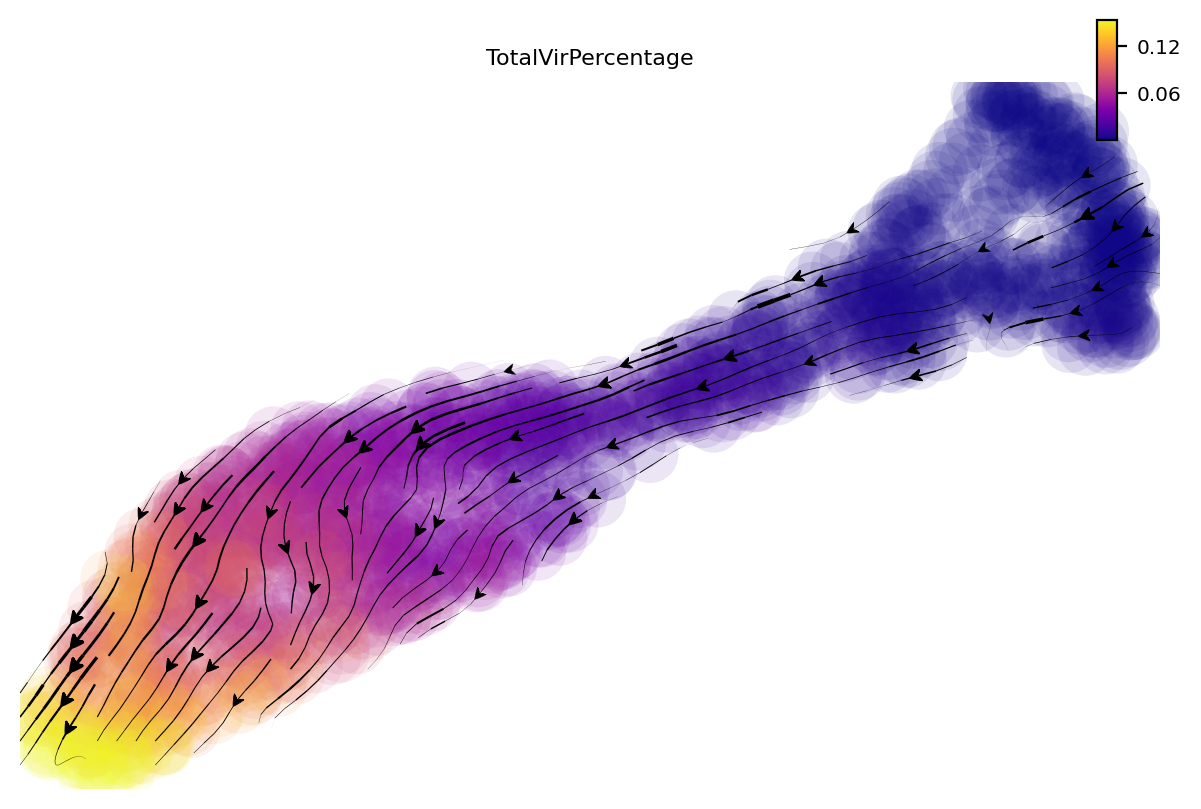
dyn.pd.perturbation(adata, 'UL112', [-100], emb_basis="umap", projection_method='cosine')
dyn.pl.streamline_plot(adata, color=['TotalVirPercentage'], basis="umap_perturbation", cmap='plasma')

|-----> In silico perturbation of single-cells and prediction of cell fate after perturbation...
|-----> Retrive X_pca, PCs, pca_mean...
|-----> Calculate perturbation effect matrix via \delta Y = J \dot \delta X....

calculating Jacobian for each cell: 100%|██████████| 1454/1454 [00:00<00:00, 299607.86it/s]

|-----> project the pca perturbation vector to low dimensional space....
|-----> [calculating transition matrix via cosine kernel with sqrt transform.] in progress: 5.1582%

|-----> [calculating transition matrix via cosine kernel with sqrt transform.] in progress: 100.0000%|-----> [calculating transition matrix via cosine kernel with sqrt transform.] completed [0.3061s]
|-----> [projecting velocity vector to low dimensional embedding] in progress: 100.0000%|-----> [projecting velocity vector to low dimensional embedding] completed [0.2248s]
|-----> method arg is None, choosing methods automatically...
|-----------> method kd_tree selected
|-----> you can use dyn.pl.streamline_plot(adata, basis='umap_perturbation') to visualize the perturbation vector
|-----> method arg is None, choosing methods automatically...
|-----------> method kd_tree selected
|-----------> plotting with basis key=X_umap_perturbation

../../_images/graphvelo_notebooks_tutorials_tutorial_hcmv_25_5.png